Plotting Dendrograms
Once you have computed a dendrogram, you will likely want to plot it as well as over-plot the structures on your original image.
Interactive Visualization
One you have computed your dendrogram, the easiest way to view it interactively
is to use the viewer() method:
d = Dendrogram.compute(...)
v = d.viewer()
v.show()
This will launch an interactive window showing the original data, and the dendrogram itself. Note that the viewer is only available for 2 or 3-d datasets. The main window will look like this:
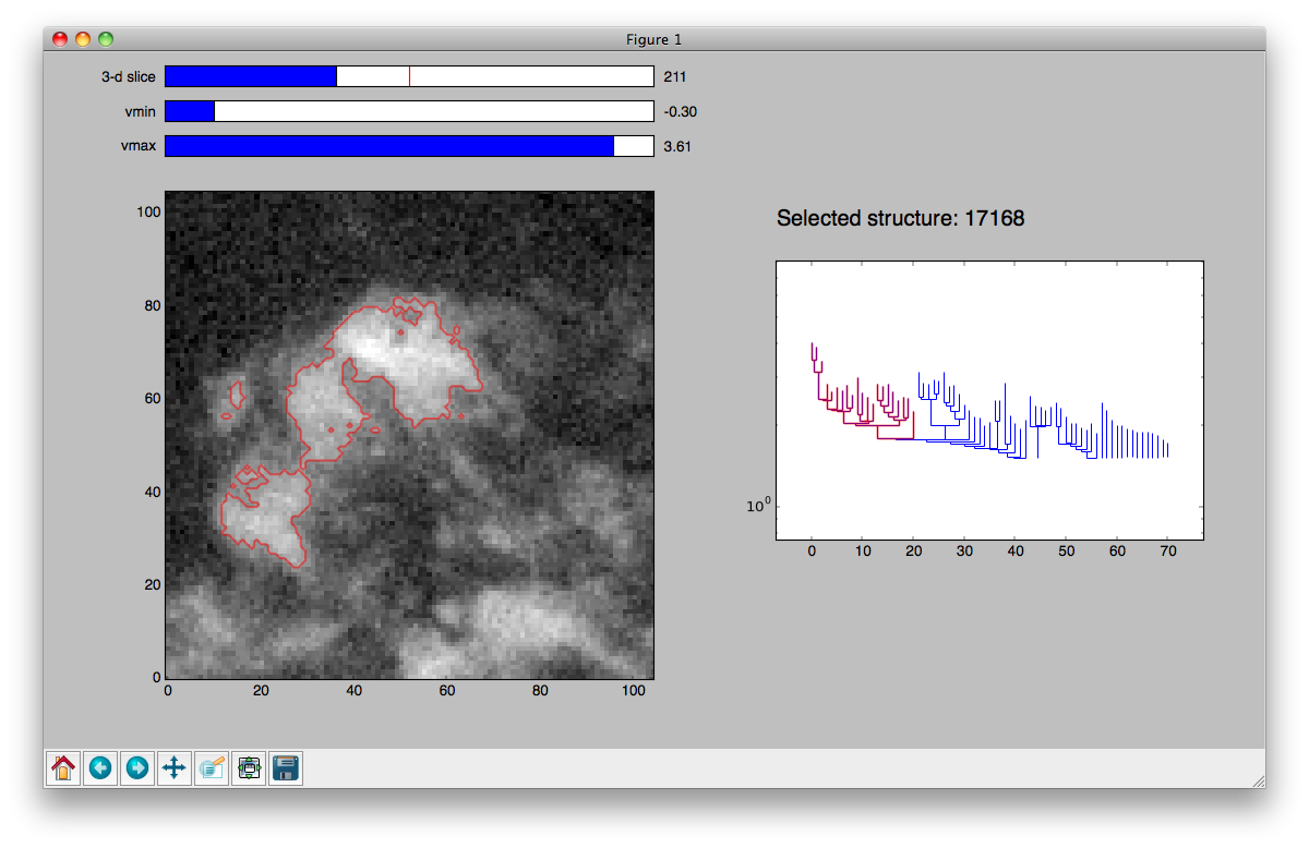
Within the viewer, you can:
Highlight structures: either click on structures in the dendrogram to highlight them, which will also show them in the image view on the left, or click on pixels in the image and have the corresponding structure be highlighted in the dendrogram plot. Clicking on a branch in the dendrogram plot or in the image will highlight that branch and all sub-structures.
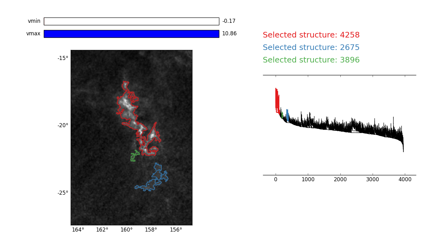
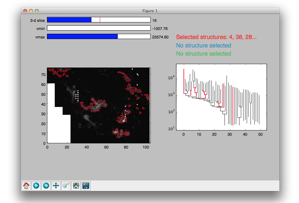
Multiple structures can be highlighted in different colors using the three mouse buttons: Mouse button 1 (Left-click or “regular” click), button 2 (Middle-click or “alt+click”), and button 3 (Right-click/”ctrl+click”). Each selection is independent of the other two; any of the three can be selected either by clicking on the image or the dendrogram.
Change the image stretch: use the vmin and vmax sliders above the
image to change the lower and upper level of the image stretch.
Change slice in a 3-d cube: if you select a structure in the dendrogram for
a 3-d cube, the cube will automatically change to the slice containing the peak
pixel of the structure (including sub-structures). However, you can also change
slice manually by using the slice slider.
View the selected structure ID: in a computed dendrogram, every structure
has a unique integer ID (the .idx attribute) that can be used to recognize
the identify the structure when computing catalogs or making plots manually
(see below).
Display astronomical coordinates:
If your data has an associated WCS object (for example, if you loaded your data
from a FITS file with astronomical coordinate information), the interactive viewer
will display the coordinates using wcsaxes:
from astropy.io.fits import getdata
from astropy import wcs

data, header = getdata('astrodendro/docs/PerA_Extn2MASS_F_Gal.fits', header=True)
wcs = wcs.WCS(header)
d = astrodendro.Dendrogram.compute(data, wcs=wcs)
v = d.viewer()
v.show()
Note that this functionality requires that the wcsaxes package is installed.
Installation instructions can be found here:
http://wcsaxes.readthedocs.org/en/latest/
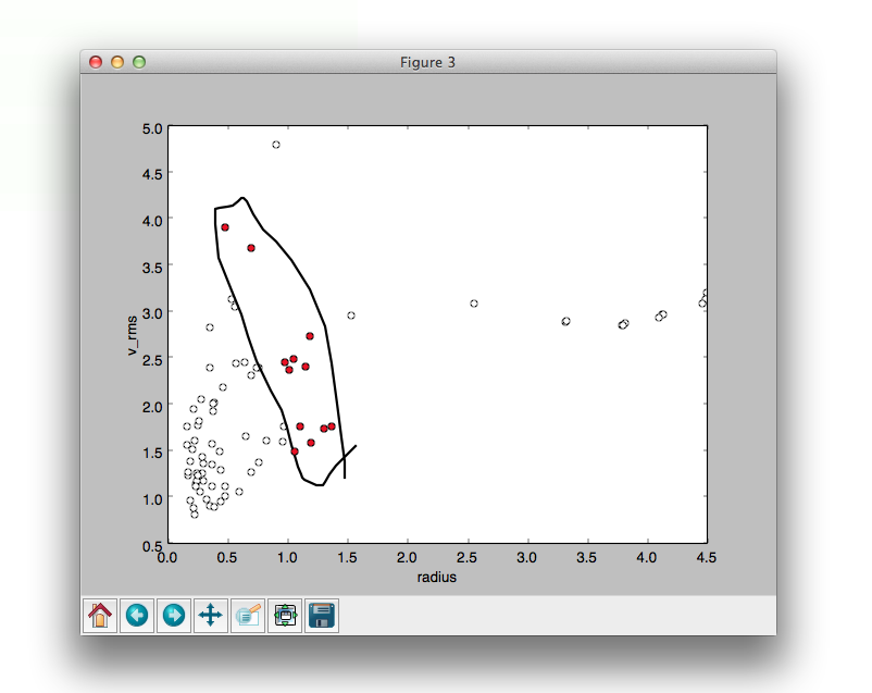
Linked scatter plots:
If you have built a catalog (see Computing Dendrogram Statistics), you can also
display a scatterplot of two catalog columns, linked to the viewer.
The available catalog columns can be accessed as `catalog.colnames`.
Selections in the main viewer update the colors of the points in this plot:
from astrodendro.scatter import Scatter
... code to create a dendrogram (d) and catalog ...
dv = d.viewer()
ds = Scatter(d, dv.hub, catalog, 'radius', 'v_rms')
dv.show()
The catalog properties of dendrogram structures will be plotted here. You can select structures directly from the scatter plot by clicking and dragging a lasso, and the selected structures will be highlighted in other plots:
To set logarithmic scaling on either the x axis, the y axis, or both, the following convenience methods are defined:
ds.set_semilogx()
ds.set_semilogy()
ds.set_loglog()

# To unset logarithmic scaling, pass `log=False` to the above methods, i.e.
ds.set_loglog(False)
Making plots for publications
While the viewer is useful for exploring the dendrogram, it does not allow one
to produce publication-quality plots. For this, you can use the non-interactive
plotting interface. To do this, you can first use the
plotter() method to provide a plotting
tool:
d = Dendrogram.compute(...)
p = d.plotter()
and then use this to make the plot you need. The following complete example
shows how to make a plot of the dendrogram of the extinction map of the Perseus
region (introduced in Computing and exploring dendrograms) using
plot_tree(), highlighting two of the
main branches:
 import matplotlib.pyplot as plt
 from astropy.io import fits
 from astrodendro import Dendrogram

 image = fits.getdata('PerA_Extn2MASS_F_Gal.fits')
 d = Dendrogram.compute(image, min_value=2.0, min_delta=1., min_npix=10)
 p = d.plotter()

 fig = plt.figure()
 ax = fig.add_subplot(1, 1, 1)

 # Plot the whole tree
 p.plot_tree(ax, color='black')

 # Highlight two branches
 p.plot_tree(ax, structure=8, color='red', lw=2, alpha=0.5)
 p.plot_tree(ax, structure=24, color='orange', lw=2, alpha=0.5)

 # Add axis labels
 ax.set_xlabel("Structure")
 ax.set_ylabel("Flux")


.. image:: _build/plot_directive/plotting-1.png
   :class: ['plot-directive']


.. image:: _build/plot_directive/plotting-1.pdf


.. image:: _build/plot_directive/plotting-1.png
   :class: ['plot-directive']
You can find out the structure ID you need either from the interactive viewer
presented above, or programmatically by accessing the idx attribute of a
Structure.
A plot_contour() method is also
provided to outline the contours of structures. Calling
plot_contour() without any arguments
results in a contour corresponding to the value of min_value used being
shown.
 import matplotlib.pyplot as plt
 from astropy.io import fits
 from astrodendro import Dendrogram

 image = fits.getdata('PerA_Extn2MASS_F_Gal.fits')
 d = Dendrogram.compute(image, min_value=2.0, min_delta=1., min_npix=10)
 p = d.plotter()

 fig = plt.figure()
 ax = fig.add_subplot(1, 1, 1)
 ax.imshow(image, origin='lower', interpolation='nearest', cmap=plt.cm.Blues, vmax=4.0)

 # Show contour for ``min_value``
 p.plot_contour(ax, color='black')

 # Highlight two branches
 p.plot_contour(ax, structure=8, lw=3, colors='red')
 p.plot_contour(ax, structure=24, lw=3, colors='orange')


.. image:: _build/plot_directive/plotting-2.png
   :class: ['plot-directive']


.. image:: _build/plot_directive/plotting-2.pdf


.. image:: _build/plot_directive/plotting-2.png
   :class: ['plot-directive']
Plotting contours of structures in third-party packages
In some cases you may want to plot the contours in third party packages such as APLpy or DS9. For these cases, the best approach is to output FITS files with a mask of the structures to plot (one mask file per contour color you want to show).
Let’s first take the plot above and make a contour plot in APLpy outlining all the leaves. We can use the get_mask() method to retrieve the footprint of a given structure:
 import aplpy
 import numpy as np
 import matplotlib.pyplot as plt
 from astropy.io import fits
 from astrodendro import Dendrogram

 hdu = fits.open('PerA_Extn2MASS_F_Gal.fits')[0]
 d = Dendrogram.compute(hdu.data, min_value=2.0, min_delta=1., min_npix=10)

 # Create empty mask. For each leaf we do an 'or' operation with the mask so
 # that any pixel corresponding to a leaf is set to True.
 mask = np.zeros(hdu.data.shape, dtype=bool)
 for leaf in d.leaves:
     mask = mask | leaf.get_mask()

 # Now we create a FITS HDU object to contain this, with the correct header
 mask_hdu = fits.PrimaryHDU(mask.astype('short'), hdu.header)

 # We then use APLpy to make the final plot
 fig = aplpy.FITSFigure(hdu, figsize=(8, 6))
 fig.show_colorscale(cmap='Blues', vmax=4.0)
 fig.show_contour(mask_hdu, colors='red', linewidths=0.5)
 fig.tick_labels.set_xformat('dd')
 fig.tick_labels.set_yformat('dd')


.. image:: _build/plot_directive/plotting-3.png
   :class: ['plot-directive']


.. image:: _build/plot_directive/plotting-3.pdf


.. image:: _build/plot_directive/plotting-3.png
   :class: ['plot-directive']
Now let’s take the example from Making plots for publications and try and
reproduce the same plot. As described there, one way to find interesting
structures in the dendrogram is to use the Interactive Visualization tool.
This tool will give the ID of a structure as an integer (idx).
Because we are starting from this ID rather than a
Structure object, we need to first get the
structure, which can be done with:
structure = d[idx]
where d is a Dendrogram instance. We also
want to create a different mask for each contour so as to have complete control
over the colors:
 import aplpy
 from astropy.io import fits
 from astrodendro import Dendrogram

 hdu = fits.open('PerA_Extn2MASS_F_Gal.fits')[0]
 d = Dendrogram.compute(hdu.data, min_value=2.0, min_delta=1., min_npix=10)

 # Find the structures
 structure_08 = d[8]
 structure_24 = d[24]

 # Extract the masks
 mask_08 = structure_08.get_mask()
 mask_24 = structure_24.get_mask()

 # Create FITS HDU objects to contain the masks
 mask_hdu_08 = fits.PrimaryHDU(mask_08.astype('short'), hdu.header)
 mask_hdu_24 = fits.PrimaryHDU(mask_24.astype('short'), hdu.header)

 # Use APLpy to make the final plot
 fig = aplpy.FITSFigure(hdu, figsize=(8, 6))
 fig.show_colorscale(cmap='Blues', vmax=4.0)
 fig.show_contour(hdu, levels=[2.0], colors='black', linewidths=0.5)
 fig.show_contour(mask_hdu_08, colors='red', linewidths=0.5)
 fig.show_contour(mask_hdu_24, colors='orange', linewidths=0.5)
 fig.tick_labels.set_xformat('dd')
 fig.tick_labels.set_yformat('dd')


.. image:: _build/plot_directive/plotting-4.png
   :class: ['plot-directive']


.. image:: _build/plot_directive/plotting-4.pdf


.. image:: _build/plot_directive/plotting-4.png
   :class: ['plot-directive']